Note: phiên bản Tiếng Việt của bài này ở link dưới.

https://duongnt.com/adversarial-example-vie

When properly trained on a good dataset, a deep learning model can achieve seemingly superhuman accuracy. But at the end of the day, it is still just a bunch of mathematical equations. By applying the same process used in training, we can craft examples that are obvious to humans but can fool a deep learning model. Today, we will try to create such adversarial examples using Tensorflow.

You can download all sample code from the link below.

https://gist.github.com/duongntbk/8cbb78b49264bcf0262d3856d04e6fec

The model we try to fool

We will try to fool the gender prediction model trained in a previous article. You can download the model from this link.

We also need a base image, let’s use my picture below. Notice that I resized it to 150×150 pixels so that we don’t have to rescale it again before feeding it to our model.

Recall that our model reached ~91% accuracy on the test dataset. We can verify that it can predict the correct gender for the original image.

model_path = 'gender_prediction_best.keras'
model = load_model(model_path)

image_path = 'adversarial-example-origin.png'
image = load_img(image_path, target_size=(150, 150), interpolation='bilinear')
image = img_to_array(image, data_format='channels_last') / 255.0
image = image.reshape(1, 150, 150, 3)

pred = model.predict(image) # Return 0.000004351216

Because our model use 0 to label male and 1 to label female, the result above means our model thinks the original image is male with 99.9995648784% certainty.

Overview of the fast sign gradient method (FSGM)

Just like the training process of a deep learning model, FSGM also uses the stochastic gradient descent method. The only difference is the loss value we try to minimize.

• In a normal training process: the loss value measures how close the model’s prediction is to the actual label of a data point.
• In FSGM: the loss value measures how close the model’s prediction to a label we choose (not necessarily the correct one).

Since our model is a two-class classifier, its output is a floating point number between 0 and 1. The closer that number is to 0, the more likely that the input belongs to class 0, and vice versa. Because of that, to create an adversarial example based on our original image, we can define the loss value as how close the model’s prediction is to 1.

Thus, the steps to perform FSGM are below.

• Use the target model to classify the original image. The result is a number very close to 0.
• Calculate 1-result and use it as our loss value. At first, the loss is close to 1.
• Calculate the gradient of the loss value based on the origin image.
• Adjust the value of the original image in the opposite direction of the gradient.
• Repeat the steps above until the loss value is small enough.

Apply FSGM to our model and original image

Calculate the gradient of loss value

The first step is to convert our image into a variable tensor. This is necessary because we want to update our image after each training step based on the loss gradient.

tensor = tf.Variable(image)

Tensorflow makes calculating a gradient very simple, all we need is a GradientTape object.

with tf.GradientTape() as tape:
    tape.watch(tensor)
    loss = 1 - model(tensor)

grad = tape.gradient(loss, tensor) # Calculate the gradient of the loss value based on the input tensor

Running the code above gives us the following result.

array([[[[-6.51887875e-12,  1.98002892e-10,  3.26648486e-10],..., dtype=float32)
dtype:dtype('float32')
max:2.1715496e-06
min:-3.3731865e-06
shape:(1, 150, 150, 3)
size:67500

Define a training step

Given the gradient above, it’s simple to define our training step as below.

def training_step(tensor, learning_rate):
    with tf.GradientTape() as tape:
        tape.watch(tensor)
        loss = 1 - model(tensor)

    grad = tape.gradient(loss, tensor) # Calculate the gradient of the loss value based on the input tensor
    tensor.assign_sub(grad * learning_rate)
    return loss

An important question is what learning rate should we use? From the previous section, we can see that our gradient is very small, its values are in the range [-3.3731865e-06, 2.1715496e-06]. If we use a learning rate in the [1e-4, 1e-3] range as usual, our training will proceed very slowly. Since the input tensor has values in the [0, 1] range, I think we should adjust it by 1e-4 or so every step. Let’s set our learning rate to 50 for now.

The code to set up the training loop is below.

learning_rate = 50
epsilon = 1e-4
for i in range(1000): # perform 1000 steps
    loss = training_step(tensor, learning_rate)

    if loss < epsilon: # Stop training if loss is smaller than epsilon
        print(f'Stop training at step {i}/1000: loss={loss}.')
        break

    if i % 25 == 0: # Print loss value every 25 steps
        print(f'Step {i}/1000: loss={loss}.')

First attempt

After 1000 steps, we run the modified image through our model.

faked = tensor.numpy()
faked = np.clip(faked, 0, 1) # Normalize the modified image into the [0, 1] range

pred = model.predict(faked) # Return 1

Our model is now 100% certain that the modified image is female. But did we really succeed? Let’s view the modified image.

faked = faked.reshape(150, 150, 3)
plt.imshow(faked)
plt.show()

Yikes, the result does not look too good. There are a lot of artifacts, and the color also looks all weird. I think we can do better.

Where did we go wrong?

Let’s look at the loss value in our previous training.

Step 0/1000: loss=[[0.99999565]].
Step 25/1000: loss=[[0.9999919]].
Step 50/1000: loss=[[0.99994403]].
Stop training at step 57/1000: loss=[[0.]].

By step 50, the loss value is still close to 1, yet by step 57 it has fallen to 0. This sudden drop in loss value makes me question our current learning rate. Let’s add some code to retrieve the minimum and maximum gradient values for each step.

def training_step(tensor, learning_rate):
    with tf.GradientTape() as tape:
        tape.watch(tensor)
        loss = 1 - model(tensor)
    grad = tape.gradient(loss, tensor)
    grad_max = tf.math.reduce_max(grad).numpy() # Find the gradient's maximum value.
    grad_min = tf.math.reduce_min(grad).numpy() # Find the gradient's minimum value.

    tensor.assign_sub(grad * learning_rate)
    return loss, grad_max, grad_min

And we will display those values along with the loss for all steps after step 50.

for i in range(1000):
    loss, grad_max, grad_min = training_step(tensor, learning_rate)
    if loss < 1e-4:
        break
    if i >= 50: # Print loss and maximum/minimum gradient from step 50
        print(f'Step {i}/1000: loss={loss}. Maximum gradient: {grad_max}. Minimum gradient: {grad_min}')

Below is the result.

Step 50/1000: loss=[[0.99994403]]. Maximum gradient: 2.601052801765036e-05. Minimum gradient: -3.883903264068067e-05
Step 51/1000: loss=[[0.99992836]]. Maximum gradient: 3.351546547492035e-05. Minimum gradient: -5.5405471357516944e-05
Step 52/1000: loss=[[0.99990195]]. Maximum gradient: 4.4642067223321646e-05. Minimum gradient: -6.508854130515829e-05
Step 53/1000: loss=[[0.99984944]]. Maximum gradient: 7.057357288431376e-05. Minimum gradient: -0.00010238249524263665
Step 54/1000: loss=[[0.9997081]]. Maximum gradient: 0.00014037966320756823. Minimum gradient: -0.000200723807211034
Step 55/1000: loss=[[0.9989778]]. Maximum gradient: 0.00045278333709575236. Minimum gradient: -0.0007489514537155628
Step 56/1000: loss=[[0.9643442]]. Maximum gradient: 0.020121416077017784. Minimum gradient: -0.026629919186234474

We can clearly see that after step 53, the gradient’s absolute values grow rapidly. And because we fix our learning rate at 50, we will make very large changes to the original image. This can explain all the artifacts and weird color patches in our final result.

Implement a crude adaptive learning rate

Ideally, we want to start with a relatively big learning rate, then reduce it little by little as the gradient becomes bigger. We will choose the learning rate so that at each step we modify the original image by no more than 1e-3.

MAX_CHANGE = 1e-3

def calculate_lr(grad_max, grad_min, max_change=MAX_CHANGE):
    max_abs_grad = max(np.abs(grad_min), np.abs(grad_max))
    return max_change / max_abs_grad

def training_step(tensor):
    with tf.GradientTape() as tape:
        tape.watch(tensor)
        loss = 1 - model(tensor)
    grad = tape.gradient(loss, tensor)
    grad_max = tf.math.reduce_max(grad).numpy()
    grad_min = tf.math.reduce_min(grad).numpy()

    learning_rate = calculate_lr(grad_max, grad_min) # Tune the learning rate at each step
    tensor.assign_sub(grad * learning_rate)
    return loss

epsilon = 1e-4
for i in range(1000): # perform 1000 steps
    loss = training_step(tensor)

    if loss < epsilon: # Stop training if loss is smaller than epsilon
        print(f'Stop training at step {i}/1000: loss={loss}.')
        break

    if i % 25 == 0: # Print loss value every 25 steps
        print(f'Step {i}/1000: loss={loss}.')

This time, the result looks much better.

But did we fool our model?

faked = tensor.numpy()
faked = np.clip(faked, 0, 1) # Normalize the modified image into the [0, 1] range

pred = model.predict(faked) # Return 0.99962485

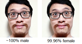
Our model is 99.96% certain that the modified image is female. I would say that we have thoroughly fooled it.

As a final comparison, below is the original image and the modified image side by side. I cannot see any difference between them, can you?

Conclusion

At first glance, it seems that a deep learning model is an impenetrable black box. But if we understand the training process, we can easily confuse it. FSGM is a simple algorithm, but there are much more sophisticated ones, such as LinfDeepFoolAttack or NewtonFool.